Musical Gestures Toolbox for Python - Tutorial

Introduction

The Musical Gestures Toolbox for Python is a collection of tools for video visualization and video analysis. It also has some modules for audio analysis and will be developed to include integration with motion capture and sensor data.

The tools are developed for video material shot with a camera placed on a tripod and with a stable background and lighting.

This tutorial will go through some of the core parts of the toolbox. Please refer to the Wiki for details.

History

The toolbox builds on the Musical Gestures Toolbox for Matlab, which again builds on the Musical Gestures Toolbox for Max.

We have also developed the standalone software VideoAnalysis for those that are not into programming.

Development

The software is developed by researchers at the fourMs lab at RITMO Centre for Interdisciplinary Studies in Rhythm, Time and Motion at the University of Oslo.

Feel free to contribute to the code at GitHub!

It is also great if you can log bugs and feature requests in the Issues section.

Setting up

We assume that you have a functioning version of Python and Jupyter Notebook running on your system.

You can install the toolbox using this terminal command:

!pip install musicalgestures

Using Google Colab

If you don't have your system setup properly, you can try it in your browser using Google Colab.

First, let's download and install the module:

!pip install musicalgestures

If you are prompted to restart the runtime, do so by clicking the button in the previous cell. This is necessary if the required version of IPython is newer than the one that is preinstalled on Colab.

Now we should install a relatively new version of FFmpeg (again, we need a bit newer one than what comes with Colab). First we add a repository that has the newer version, and then we download and install it.

!add-apt-repository -y ppa:jonathonf/ffmpeg-4
!apt install --upgrade ffmpeg

Importing

In Jupyter Notebook, we start by importing the toolbox using the command musicalgestures and make a "shortcut" with the command mg:

import musicalgestures as mg

To make your first steps a bit easier, we packaged a couple of example videos into musicalgestures. We load them into two variables:

dance = mg.examples.dance

pianist = mg.examples.pianist

Loading a video file

Now we can load one of the video files into a video object:

video = mg.MgVideo(dance)

Now the video object contains a pointer to the video file and it is also "actionable".

Watching a video file

You can watch your video with calling the show() method. There are two modes to choose from:

1. The default 'windowed' mode will open a video player as a separate window.
2. The 'notebook' mode the video is embedded into the notebook.

video.show() # this opens the video in a separate window

video.show(mode="notebook") # this embeds the video in the notebook

Since only mp4, webm and ogg file formats are compatible with browsers, show will automatically convert your video to mp4 if necessary. Please note that the notebook-mode will not work in Colab.

Preprocessing modules

Trimming

It is possible to trim the video, that is, select its start and end time. This is specified in the unit of seconds:

video = mg.MgVideo(dance, starttime=5, endtime=15)

This function will create the file dance_trim.avi in the same directory as the video file.

The file can then be shown like this:

video.show()

Skipping

Skipping frames in the video can reduce the analysis time. You can skip frames between every analysed frame by using the skip function:

video = mg.MgVideo(dance, skip=5)
video.show()

This will create the file dance_skip.avi in the same directory. Notice how the added suffixes at the end of the file's name can inform you about the processes the material went through. If a similar file already exists, it will add an incremental number to avoid overwriting existing files.

Rotating

Some videos are recorded slightly tilted, or with the camera mounted sideways.

We can rotate the video 90 degrees with the rotate parameter:

video = mg.MgVideo(dance, starttime=5, endtime=15, skip=3, rotate=90)
video.show()

Or with some other angle:

video = mg.MgVideo(dance, starttime=5, endtime=15, skip=3, rotate=3.3)
video.show()

Again, the resulting filename dance_trim_skip_rot.avi will inform us about the chain of processes dance.avi went through.

Adjusting contrast and brightness

During preprocessing you can also add (or remove) some contrast and brightness of the video:

video = mg.MgVideo(dance, starttime=5, endtime=15, contrast=100, brightness=20)
video.show()

The resulting file is now called dance_trim_skip_rot_cb.avi.

Cropping

You may not be interested in analysing the whole image. Then it is helpful to crop the video. This can be done manually by clicking and selecting the area to crop followed by pressing the key c:

video = mg.MgVideo(dance, starttime=5, endtime=15, crop='manual')
video.show()

There is also an experimental "auto-crop" function that looks at where there motion in the video at uses that for cropping:

video = mg.MgVideo(dance, starttime=5, endtime=15, crop='auto')
video.show()

This may or may not work well, dependent on the content of the video.

Grayscale mode

If you do not need to work with colors, you may speed up the further processing considerably (3x) by converting to grayscale mode using the color=False command:

video = mg.MgVideo(dance, starttime=5, endtime=15, skip=3, color=False)
video.show()

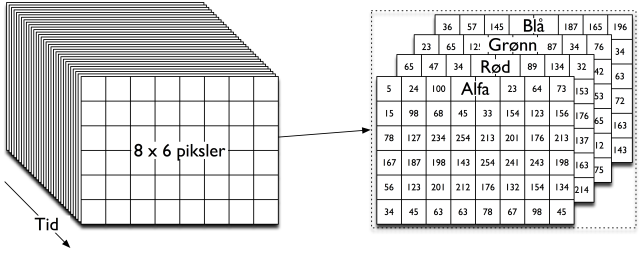
A color video is composed of 4 planes (Alpha, Red, Green, Blue) while a grayscale only has one. This is why the further analysis will be reduced to 1/4 in computational needs.

Summary of preprocessing modules

These are the six preprocessing steps we have used so far:

• trim: Trim the beginning and end of the video
• skip: Skip every n frames to reduce processing time
• rotate: Rotate the video by an angle
• cb: Adjust contrast and brightness
• crop: Crop out a part of the video image
• grayscale: Convert the video to grayscale to reduce processing time

It's a chain

Note that the preprocessing modules work as a chain:

1. load the file
2. trim its start to 5s and its end to 15s
3. skip 2 frames (keeping the 1st, skipping 2nd and 3rd, keeping the 4th, skipping 5th and 6th, and so on...)

The resulting file of this process is dance_trim_skip.avi.

Keep everything

The toolbox has been designed to store new video files for each chain.

You can optionally keep the video files for each part of the chain by setting keep_all=True:

video = mg.MgVideo(dance, starttime=5, endtime=15, skip=3, rotate=3, contrast=100, brightness=20, crop='auto', color=False, keep_all=True)

This will output six new video files:

• dance_trim.avi
• dance_trim_skip.avi
• dance_trim_skip_rot.avi
• dance_trim_skip_rot_cb.avi
• dance_trim_skip_rot_cb_crop.avi
• dance_trim_skip_rot_cb_crop_gray.avi

Video visualization

In the following we will take a look at several video processing functions:

• grid(): Creates a grid-based image with multiple frames
• videograms(): Outputs the videograms in two directions
• history(): Renders a _history video by layering the last n frames on the current frame for each frame in the video
• average(): Renders an _average image of all frames in the video

Grid image

The grid function generates an image composed of a specified number of frames sampled from the video. It gives an overview of the content of the file.

video_grid = video.grid(height=300, rows=1, cols=9)
video_grid.show(mode='notebook')

video_grid = video.grid(height=300, rows=3, cols=3)
video_grid.show(mode='notebook')

Average image

You can also summarize the content of a video by showing the average of all frames in a single image.

video.average().show(mode='notebook')

This resembles an "open shutter" technique used in early photography, blending all images together.

History video

A history video preserves somes information about previous frames through a delay process. The last n frames overlaid on top of the current one.

history = video.history(history_length=30) # returns an MgVideo with the history video
history.show()

Such history videos can be useful to display the trajectories of motion over time.

It can also be the input to a grid image:

video_grid = history.grid(height=300, rows=3, cols=3)
video_grid.show(mode='notebook')

Videograms

A videogram is a compact representation based on summing up either the rows or columns of the video.

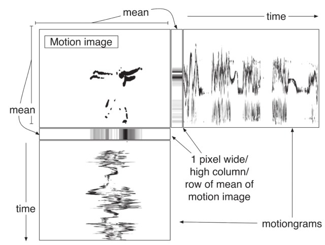
Videograms can be created using the videograms() function:

videograms = video.videograms()

videograms.show() # view both videograms

videograms[0].show() # view vertical videogram

videograms[1].show(mode="notebook") # view horizontal videogram

They are useful for getting an overview over longer video recordings, anything from minutes to hours of material. The dimensions of the output image are based on the pixels and frames of the source video. You may therefore want to use the skip function when reading the video to reduce the number of frames of long videos.

Motion analysis

These processes are based on analyzing what changes in the video files.

• motion(): The most frequently used function generates a motion video, motiongrams, a data file, and plots of the data.

The motion() function encapsulates these four functions:

• motionvideo(): This function only generates a motion video
• motiondata(): This function only generates motion data
• motionplots(): This function only generats motion plots
• motiongrams(): This function only outputs the motiongrams.

After we switched to FFmpeg rendering, there is no particular performance benefit of running the processes separately.

Frame differencing

The motion() function does many things at once. It is based on the concept of "frame differencing".

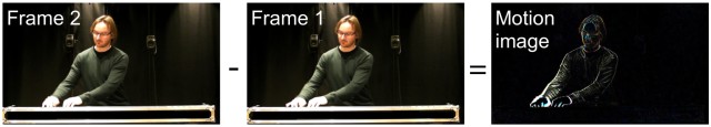
Only pixels that change between frames are shown.

video.motionvideo().show()

Motiongrams

Motiongrams are based on the same processing as videograms but starting from a motion video.

Motiongrams are created with the motiongram() function:

motiongrams = video.motiongrams()

motiongrams[0].show()

motiongrams[1].show(mode="notebook") # view horizontal videogram

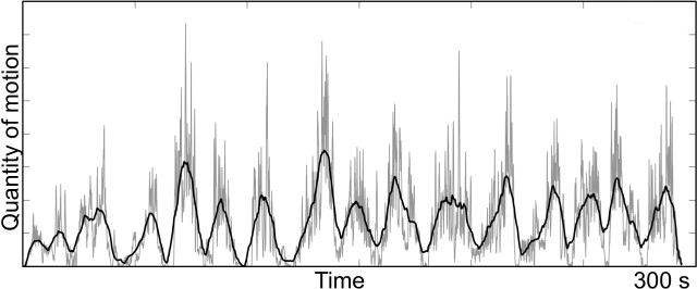
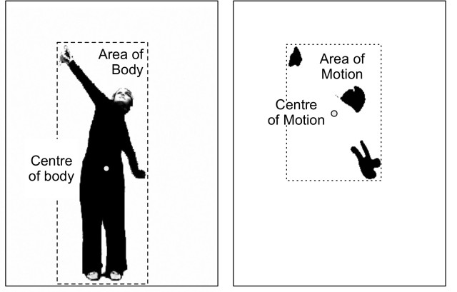
Motion features

We can extract some basic features from the motion video:

• Quantity of Motion (QoM)
• Area of Motion (AoM)
• Centroid of Motion (CoM)

Quantity of Motion

Area and centroid of motion

The features can be extracted with this command:

video.motiondata()

And plotted like this:

video.motionplots().show()

All at once

To save processing time, we have packaged many of these functions together in motion():

video.motion()

That function outputs all of these a the same time:

• _motion.avi: The motion video that is used as the source for the rest of the analysis.
• _mgx.png: A horizontal motiongram.
• _mgy.png: A vertical motiongram.
• _motion_com_qom.png: An image file with plots of centroid and quantity of motion
• _motion.csv: A text file with data from the analysis

Filtering

If there is too much noise in the output images or video, you may choose to use some other filter settings:

• Regular turns all values below thresh to 0.
• Binary turns all values below thresh to 0, above thresh to 1.
• Blob removes individual pixels with erosion method.

Finding the right threshold value is crucial for accurate motion extraction. Let's see a few examples.

First we import an example video.

video = mg.MgVideo(dance, starttime=5, endtime=10, skip=0, contrast=100, brightness=20)

First we can try to run without any threshold. This will result in a result in which much of the background noise will be visible, including traces of keyframes if the video file has been compressed.

video.motiongrams(thresh=0.0).show(mode='notebook')

Adding just a little bit of thresholding (0.02 here) will drastically improve the final result.

video.motiongrams(thresh=0.02).show(mode='notebook')

The standard threshold value (0.1) generally works well for many types of videos.

video.motiongrams(thresh=0.1).show(mode='notebook')

A more extreme value (for example 0.5) will remove quite a lot of the content, but may be useful in some cases with very noisy videos.

video.motiongrams(thresh=0.5).show(mode='notebook')

As the above examples have shown, choosing the thresholding value is important for the final output result. While it often works to use the default value (0.1), you may improve the result by testing different thresholds.

Motion history

To expressively visualize the trajectory of a moving content in a video, you can apply the history process on a motion video. You can do this by chaining motion() into history().

video.motion().history().show()

You can modify the length of the history:

video.motion().history(history_length=20).show()

And combine it with inverting the motion video:

video.motion(inverted_motionvideo=True).history().show()

Motion average

It can also be interesting to chain a motion video with the average function:

video.motion().average().show(mode="notebook")

Advanced techniques

Optical flow

It is also possible to track the direction certain points - or all points - move in a video, this is called 'optical flow'. It has two types: the sparse optical flow, which is for tracking a small (sparse) set of points, visualized with an overlay of dots and lines drawing the trajectory of the chosen points as they move in the video.

• flow.sparse(): Renders a _sparse optical flow video.
• flow.dense(): Renders a _dense optical flow video.
• pose(): Renders a _pose human pose estimation video, and optionally outputs the pose data as a csv file.

video.flow.sparse().show()

Note that sparse optical flow usually works well with slow and continuous movements, where the points to be tracked are not occluded by other objects throughout the course of motion. Where spare optical flow becomes less reliable, dense optical flow often yields more robust results. In dense optical flow the analysis attempts to track the movement of each pixel (or more precisely groups of pixels), colorcoding them with a unique color for each unique direction.

video.flow.dense().show()

Sparse optical flow can get confused by too fast movement (ie. too big distance between the locations of a tracked point between two consequtive frames), so it is typically advised not to have a too high skip value in the preprocessing stage for it to work properly. Dense optical flow on the other hand has issues with very slow movement, which sometimes gets below the treshold of what is considered 'a movement' resulting in a blinking video, where the more-or-less idle moments are rendered completely black. If your source video contains such moments, you can try setting skip_empty=True, which will discard all the (completely) black frames, eliminating the binking.

video.flow.dense(skip_empty=True).show()

Pose estimation

This module uses a more advanced type of computer vision, that involves a deep neural network trained by a huge dataset of images of people (courtesy of OpenPose!).

It tries to estimate their skeleton by tracking a set of "keypoints", which are joints on the body - for example "Head", "Left Shoulder", "Right Knee", etc. After the module runs you can take a look at the _pose.csv dataset, that contains the normalized XY pixel coordinates of each keypoint, and you can visualize the result with drawing a skeleton overlay over your video. You can choose from three trained models: the MPI (which is trained on the Multi-Person Dataset), the COCO model (trained on the COCO Dataset) or the BODY25 model. The module also supports GPU-acceleration, so if you have compiled openCV with CuDNN support, you can make the - otherwise rather slow - inference process run over 10 times faster!

The models

Since both models are quite large (~200MB each) they do not "ship" with the musicalgestures package, but we do include some convenience bash/batch scripts do download them on the fly if you need them. If the pose() module cannot find the model you asked for it will offer you to download it.

Downsampling

Running inference on large neural networks to process every pixel of every frame of your video is quite a costly operation. There is a trick however to reduce the load and this is downsampling your input image. Often times a large part of the frame is redundant and the posture of the person in the video can easily be understood on a lower resolution image as well. Downsampling can greatly speed up pose(), but of course it can also make its estimation less accurate if overused. The default value we use in pose() is downsampling_factor=2 which produces a video with one-fourth of its original resolution before feeding it to the network.

Confidence threshold

The networks are not always equally confident about their guesses. Sometimes (especially with heavy downsampling) they can identify other objects in your scene as either of the keypoints of the human body we wish to track. Filtering out inconfident guesses can remove a lot of noise from the prediction. pose() has a normalized threshold parameter that is set to 0.1. This means the network has to be at least 10% sure about its guess for us to take that prediction into account.

Below you can find a simple example of pose() in action. For more info check out the documentation.

video.pose(downsampling_factor=1, threshold=0.05, model='mpi', device='gpu').show(mode='notebook')

Audio

MGT offers several tools to analyze the audio track of videos or audio files. These are implemented both as class methods for MgObject and standalone functions.

• audio.waveform(): Renders a figure showing the waveform of the video/audio file.
• audio.spectrogram(): Renders a figure showing the mel-scaled spectrogram of the video/audio file.
• audio.descriptors(): Renders a figure of plots showing spectral/loudness descriptors, including RMS energy, spectral flatness, centroid, bandwidth, rolloff of the video/audio file.
• audio.tempogram(): Renders a figure with a plots of onset strength and tempogram of the video/audio file.

These functions use the librosa package for audio analysis and the matplotlib package for showing the analysis as figures.

Waveforms

A waveform is a plot of audio samples (y axis) against time (x axis). It is a basic visualization of the audio content. Here is how you can create a waveform of an audio track/file:

video = mg.MgVideo(pianist)
waveform = video.audio.waveform()
waveform.show()

Spectrograms

A spectrogram is a plot of frequency spectrum (y axis) against time (x axis). It can provide a much more descriptive representation of audio content than a waveform (which is in a way the sum of all frequencies with respect to their phases). Here is how you can create a spectrogram of an audio track/file:

video = mg.MgVideo(pianist)
spectrogram = video.audio.spectrogram()
spectrogram.show()

This has created a figure showing the mel-scaled spectrogram, and rendered dance_spectrogram.png in the same folder where our input video, dance.avi resides.

Tempograms

Tempograms attempt to use the same technique (called Fast Fourier Transform) as spectrograms to estimate musical tempo of the audio. In tempogram() we analyze the onsets and their strengths throughout the audio track, and then estimate the global tempo based on those. Here is how to use it:

video = mg.MgVideo(pianist)
tempogram = video.audio.tempogram()
tempogram.show()

Estimating musical tempo meaningfully is a tricky thing, as it is often a function of not just onsets (beats), but the underlying harmonic structure as well. tempogram() only relies on onsets to make its estimation, which can in some cases identify the most common beat frequency as the "tempo" (rather than the actual musical tempo).

Descriptors

Additionally to spectrograms and tempogams you can also get a collection of audio descriptors via descriptors(). This collection includes:

• RMS energy,
• spectral flatness,
• spectral centroid,
• spectral bandwidth,
• and spectral rolloff.

RMS energy is often used to get a perceived loudness of the audio signal. Spectral flatness indicates how flat the graph of the spectrum is at a given point in time. Noisier signals are more flat than harmonic ones. The spectral centroid shows the centroid of the spectrum, spectral bandwidth marks the the frequency range where power drops by less than half (at most −3 dB). Spectral rolloff is the frequency below which a specified percentage of the total spectral energy, e.g. 85%, lies. descriptors() draws two rolloff lines: one at 99% of the energy, and another at 1%.

video = mg.MgVideo(pianist)
descriptors = video.audio.descriptors()
descriptors.show()

Self-similarity matrices

Self-Similarity Matrices allow for detecting periodicities in a signal.

video = mg.MgVideo(pianist)
chromassm = video.ssm(features='chromagram', cmap='magma', norm=2) # returns an MgImage with the chromagram SSM
chromassm.show() # view chromagram SSM

Figures and Plotting

The Musical Gestures Toolbox includes several tools to extract data from audio-visual content, and many of these tools output figures (or images) to visualize this time-varying data. In this section we take a closer look on how we can customize and combine figures and images from the toolbox.

Titles

By default the figures rendered by the toolbox automatically get the title of the source file we analyzed. We can also change this by providing a title as an argument to the function or method we are using. Here are some examples:

# source video as an MgObject
video = mg.MgVideo(pianist)

# motion plots
motionplots = video.motionplots(title='Liszt - Mephisto Waltz No. 1 - motion')

# spectrogram
spectrogram = video.audio.spectrogram(title='Liszt - Mephisto Waltz No. 1 - spectrogram')

# tempogram
tempogram = video.audio.tempogram(title='Liszt - Mephisto Waltz No. 1 - tempogram')

# descriptors
descriptors = video.audio.descriptors(title='Liszt - Mephisto Waltz No. 1 - descriptors')

Combining figures and images

In this section we take a look at how we can compose time-aligned figures easily within the Musical Gestures Toolbox.

Helper data structures: MgFigure and MgList

First let us take a look at the data structures which help us through the composition.

MgFigure

As we have MgVideo for videos and MgImage for images, we also use a dedicated data structure for matplotlib figures: the MgFigure. Normally, you don't need a custom data-structure to just deal with a figure, but MgFigure offers an organized, comfortable way to represent the type of the figure and its data, so that we can reuse it in other figures. First of all, it implements the show() method which is used across the musicalgestures package to show the content of an object. In the case of MgFigure this will show the internal matplotlib.pyplot.figure object:

spectrogram.show()

Fun fact: as show() is implemented only for the sake of consistency here, you can achieve the same by referring to the internal figure of the MgFigure object directly:

spectrogram.figure # same as spectrogram.show()

What is more important is that each MgFigure has a figure_type attribute. This is what you see when you print (or in a notebook such as this, evaluate) them:

spectrogram

Each MgFigure object has a data attribute, where we store all the related data to be able to recreate the figure elsewhere. You never really have to interact with this attribute directly, unless you want to look under the hood:

print(spectrogram.data.keys()) # see what kind of entries we have in our spectrogram figure
print(spectrogram.data['length']) # see the length (in seconds) of the source file

You can also get the rendered image file corresponding to the MgFigure object. As an exercise, here is how you can make an MgImage of this image file and show it embedded in this notebook:

mg.MgImage(spectrogram.image).show(mode='notebook')

Another attribute of MgFigure is called layers. We will get back to this in a bit, for now let's just say that when an MgFigure object is in fact a composition of other MgFigure, MgImage or MgList objects, we have access to all those in the layers of the "top-level" MgFigure.

MgList

Another versatile tool in our hands is MgList. It works more-or-less as an ordinary list, and it is specifically designed for working with objects of the musicalgestures package. Here is an example how to use it:

from musicalgestures._mglist import MgList
liszt_list = MgList(spectrogram, tempogram)
liszt_list

MgList also implements many of the list feaures you already know:

# how many objects are there?
print(f'There are {len(liszt_list)} objects in this MgList!')

# which one is the 2nd?
print(f'The second object is a(n) {liszt_list[1]}.')

# change the 2nd element to the descriptors figure instead:
liszt_list[1] = descriptors
print(f'The second object is now {liszt_list[1]}.') # check results

# add the tempogram figure to the list:
liszt_list += tempogram
print(f'Now there are {len(liszt_list)} objects in this MgList. These are:') # check results
for element in liszt_list:
    print(element)

# fun fact: videograms() returns an MgList with the horizontal and vertical videograms (as MgImages)
videograms = musicalgestures.MgVideo(pianist).videograms()

# MgList.show() will call show() on all its objects in a succession
videograms.show()

# add two MgLists
everything = videograms + liszt_list
print('everything:', everything)

Composing figures with MgList

One of the most useful methods of MgList is as_figure(). It allows you to conveniently compose a stack of plots, time-aligned, and with a vertical order you specify. Here is an example:

fig_everything = everything.as_figure(title='Liszt - Mephisto Waltz No. 1')

Chaining

So far our workflow consisted of the following steps:

1. Creating an MgVideo which loads a video file and optionally applies some preprocessing to it.
2. Calling a process on the MgVideo.
3. Viewing the result.

Something like this:

video = mg.MgVideo(dance, starttime=5, endtime=15, skip=3)
video.motion()
video.show(key='motion')

This is convenient if you want to apply several different processes on the same input video.

The Musical Gestures Toolbox also offers an alternative workflow in case you want to apply a proccess on the result of a previous process. Although show() is not really a process (ie. it does not yield a file as a result) it can provide a good example of the use of chaining:

# this...
video.motion().show()

# ...is the equivalent of this!
video.motion()
video.show(key='motion')

It also works with images:

video.average().show()

But chaining can go further than this. How about reading (and preprocessing) a video, rendering its motion video, the motion history and the average of the motion history, with showing the _motion_history_average.png at the end - all as a one-liner?!

mg.MgVideo(dance, skip=4, crop='auto').motion().history().average().show(mode='notebook')

# equivalent without chaining
video = mg.MgVideo(dance, skip=4, crop='auto')
mm = video.motion()
mh = mm.history()
mh.average()
mh.show(key='average', mode='notebook')

Some other examples:

# rendering and viewing the motion video 
mg.MgVideo(dance, skip=4).motion().show(mode='notebook')

# rendering the motion video, the motion history video, and viewing the latter
mg.MgVideo(dance, skip=3).motion().history(normalize=True).show(mode='notebook')

# rendering the motion video, the motion average image, and viewing the latter
mg.MgVideo(dance, skip=15).motion().average().show(mode='notebook')

Summing up

Questions or comments?

• Wiki
• Issues